Customer service UNILAB

This technical note concerns heating and cooling coils with a single-phase fluid in the tubes (water, glycol mixtures, oils) and air across the fins. 

We receive several requests for clarification about the same behaviour: when the tube-side fluid works in the transition zone between laminar and turbulent flow, the same problem can have two physically possible solutions, with very different flow rates and duties.

The typical case is a calculation with an imposed fluid outlet temperature, where the program has to find the flow rate. Here we explain why this happens, which solution the program shows, and how to approach it at design stage.

1. Tube-side flow and the heat transfer coefficient

The flow regime in the tubes is identified by the Reynolds number, which is proportional to velocity and therefore to flow rate. Below about 2,000 the flow is laminar, above about 3,000-4,000 it is fully turbulent; in between lies the transition zone.

In laminar flow the tube-side heat transfer coefficient is low and grows little with flow rate. In turbulent flow it is much higher. The change happens over a narrow range of flow rate: the tube-side coefficient can rise 2-3 times with 20-25% more flow (figure 1).

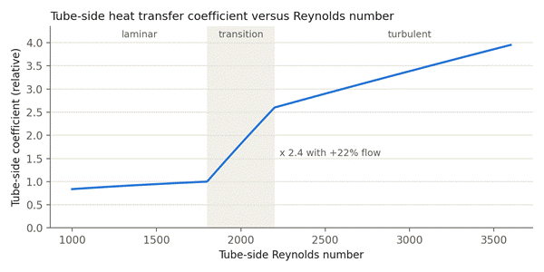
Figure 1 – Typical tube-side heat transfer coefficient (relative values, illustrative example).

2. Why there can be two operating points

The duty exchanged by the fluid must satisfy the energy balance: Q = flow rate × specific heat × (inlet T − outlet T). With a fixed outlet temperature the required duty is proportional to the flow rate: in figure 2 it is the orange line. The duty the coil can actually exchange is the blue curve.

Normally the coil curve grows more slowly than the line: more flow means an outlet temperature closer to the inlet, and the two lines meet at a single point. In the transition zone, however, the tube-side coefficient rises so fast that the coil duty grows faster than the flow rate, and the blue curve crosses the line more than once.

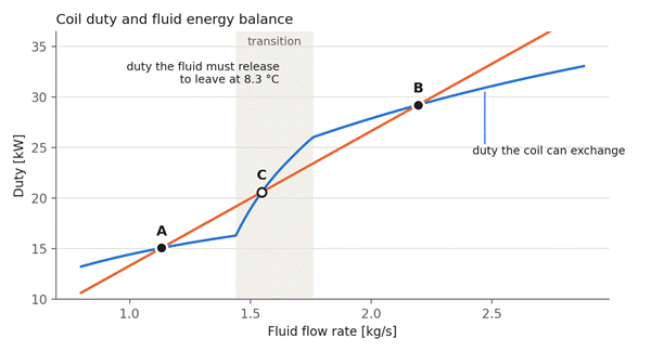
Figure 2 – Illustrative example: fluid at 12 °C, required outlet 8.3 °C. Points A, C and B all satisfy the energy balance.

The same effect is even clearer on the outlet temperature (figure 3). In laminar flow the outlet temperature rises with flow rate, as expected. In the transition zone it goes back down, because heat transfer improves faster than the flow increases. In turbulent flow it rises again. Any outlet temperature between the minimum and maximum of the curve is therefore reached with three different flow rates.

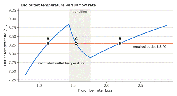
Figure 3 – Same example: the required outlet temperature is reached with three flow rates.

The effect is stronger the more the tube-side thermal resistance weighs on the total, that is with glycol mixtures, at low temperatures (more viscous fluid) and with very efficient fins. With warm water and an air-side-controlled coil it usually does not appear.

3. Which point is the real one

In the example the points are:

A and B are both physically correct: with the flow of point A the coil really exchanges 15.1 kW and the fluid leaves at 8.3 °C; with the flow of point B it exchanges 29.2 kW and the fluid still leaves at 8.3 °C. Point C falls in the transition zone, where the flow is neither laminar nor turbulent and correlations are inherently less reliable: it should not be used as a design point.

In a real plant the outlet temperature is not imposed: the pump and the circuit set the flow rate, and the outlet temperature follows. Which point actually occurs depends on the flow the plant really circulates through the coil.

4. How the program behaves

• In a calculation with imposed flow rate there is always a single solution: the program calculates duty and outlet temperature for that flow.
• In a calculation with imposed outlet temperature (unknown flow rate), when more than one solution exists the program gives priority to the one with the highest duty, i.e. the highest flow rate (point B).
• If the high-flow solution is missed by a small margin, because the minimum of the figure 3 curve stays just above the required temperature, the program shows the point at the start of turbulent flow: the outlet temperature shown can differ from the required one by a few tenths of a degree.

This is why two very similar coils, or the same coil with a small change in air flow or temperature, can give results with very different duties: one works on the turbulent branch, the other on the laminar one. It is not a calculation error: it is the physical jump between the two regimes.

5. Recommendations

• If the plant flow rate is known, use the imposed-flow calculation. The answer is unique and matches what happens in the plant.
• Check the tube-side Reynolds number shown in the results. Between about 1,800 and 3,000 the coil works close to the transition and its performance depends strongly on the flow rate.
• Avoid designing in the transition zone. Changing the number of circuits moves the tube velocity: fewer circuits push the flow firmly into turbulent (more heat transfer, more pressure drop), more circuits keep it laminar (less pressure drop, less heat transfer, but stable behaviour).
• With glycols at low temperature review concentration and mean temperature: viscosity shifts the Reynolds number considerably, and with it the position of the transition.
• Internally grooved tubes or turbulators make tube-side heat transfer less sensitive to the flow regime and soften the jump.
• Keep a margin when the operating point is close to the transition: in reality too, the change from laminar to turbulent depends on bends, headers and inlet conditions, and can happen earlier or later than the correlations predict.

6. Summary

In the transition zone between laminar and turbulent flow the tube-side heat transfer coefficient grows much faster than the flow rate. Therefore, with an imposed outlet temperature, the same coil can meet the requirement with a low flow rate in laminar flow and with a high flow rate in turbulent flow, with duties that can differ by a factor of two. Both solutions are physically possible; the program favours the one with the highest duty. For a robust design it is best to know the real plant flow rate and to choose a circuiting that keeps the fluid away from the transition.